Engineering leader building resilient, privacy-minded systems for insurance claims — and researching practical AI that earns trust at the point of decision.
Engineering systems that carry real responsibility.
Staff Engineering Manager at GEICO leading claims engineering. Previously Staff Software Engineer at Meta, end-to-end lead on the ads creation platform — shipping 1-Click Ad Creation and launches that added $35K–$50K/day in revenue, new targeting signals worth $30K/day, and Start-Your-Day upsells at $9K/day, while taking European ad privacy to compliance and lifting team SLA from 50% to 85%. At GEICO he built the company-wide mentor-mentee platform, runs org-wide PII protection at 100% compliance with zero incidents, owns BCDR across 15+ applications, and cut critical-incident MTTR 40% with AI observability. He also shipped an AI photo-integrity detector for claim fraud (Hugging Face + live demo). M.S. Computer Science, Kent State.
Current research
AI for insurance claims: photo-integrity verification for FNOL triage and multimodal severity prediction.
02 / Featured AI work
Is this claim photo authentic?
Live model · Hugging Face
Claim Photo Integrity Detector
A binary image classifier for authentic versus AI-generated or manipulated claim photos. The model fine-tunes ViT-base on Defactify data to support more trustworthy FNOL triage.
Two Groups, One Maze: Bidirectional BFS in Real Life
Two groups walked into a hay-bale maze from opposite ends and met in the middle. That's not just a fun afternoon — it's one of the most practical search algorithms there is.
The hay-bale maze where two groups, starting at opposite entrances, turned “meet in the middle” into something we could see.
I visited a botanical garden with my family, and in the middle of the fall displays they had built a big maze from stacked hay bales. Pumpkins lined the edges. Kids ran through the passages, disappearing around one corner and reappearing at another. The whole place felt busy, playful, and just uncertain enough to make choosing a direction interesting.
Our group split. One group entered from one side of the maze; another started at the entrance on the opposite side. We did not plan an algorithm. We simply began exploring inward, taking turns and checking passages. Then, somewhere in the middle, the two groups found each other.
Watching that happen, I realized we had just acted out bidirectional breadth-first search with real people in a real maze. Instead of making one group cover every promising path from a single entrance, we had two search waves moving toward each other. The meeting point connected the route.
First, picture ordinary BFS as a spreading wave
Breadth-first search, or BFS, starts where you stand and explores level by level. First it checks every place one step away, then every place two steps away, then three. Imagine dropping a pebble into still water: the ring expands evenly in every direction. In code, a queue keeps that order honest, and a visited set prevents the search from walking the same passage twice.
On an unweighted graph — where every edge counts as one step — that level-by-level discipline guarantees a shortest path. It will not wander ten turns deep while ignoring a solution only four turns away. But the wave can become enormous. If every junction offers several new choices, each level may contain many more states than the last.
01One wide wave, or two smaller waves that meet.
The twist: send a second wave from the goal
Bidirectional BFS uses the same idea twice. One search begins at the start. A second begins at the known goal and works backward. Each keeps its own frontier, visited set, and parent links. When a state visited from one side appears in the other side's visited set, the two waves have touched. Follow the parent links back toward both ends, join the two halves, and you have the complete path.
That is exactly what our groups did. One side of the hay maze was the start; the other was the goal. Every passage could be walked in either direction. When we met, we knew how to connect the entrances without asking one group to search the whole maze alone.
Don't search the whole maze from one end. Start a second search from the other end and meet in the middle.
Why half the depth changes almost everything
The advantage is not merely “two groups are twice as fast.” Search spaces grow exponentially. If each state branches to about b new states and the shortest solution is d steps deep, a one-directional BFS explores on the order of bd states. Bidirectional search asks each side to cover roughly half the distance, so the work is closer to bd/2 from each end, or about 2 · bd/2 in total.
Take a small-looking example: three choices per step and a solution ten steps away. A one-directional estimate is 310, or about 59,049 nodes. From both ends, each search travels only five levels: 2 × 35 = 2 × 243, or about 486 nodes. That is under one percent of the one-way estimate. Meeting in the middle cuts the exponent in half.
02Half the depth turns 59,049 into about 486.
When meeting in the middle works
The technique has two important requirements. First, you need to know the goal state up front; “find anything interesting” does not give the reverse search a place to begin. Second, you must be able to search backward from that goal. The moves do not always have to be physically reversible, but the algorithm needs a way to generate predecessor states. Our maze is the friendly case: both entrances are known, and every passage is walkable both ways.
In an implementation, it is also wise to expand the smaller frontier at each step. That keeps the more rapidly growing side from dominating memory. And, as with ordinary BFS, the shortest-path guarantee assumes unweighted edges; weighted roads or transitions call for bidirectional versions of Dijkstra's algorithm or A*, with more careful stopping rules.
Where engineers use it
The pattern appears anywhere a forward-only search threatens to explode. In a social graph, one wave can start from you and another from a distant person to find the shortest chain of connections — the familiar “degrees of separation.” Route-finding systems can search from origin and destination. Word ladders can grow transformations from both words. Puzzle solvers use it for spaces such as the 15-puzzle and Rubik's Cube, where the target arrangement is known and legal moves can be reversed.
The broader lesson stayed with me after the botanical garden. The fastest way through a maze — or a search space — is often not to push harder from one end. It is to start from both ends, keep the waves disciplined, and let them meet in the middle.
AI tools were used for research assistance, reference gathering, and editorial support. The author reviewed, verified, and approved the final content.
Blog · Insurance engineering
Stop Re-Sending the Claim File
The expensive part of an insurance AI assistant isn't the answer — it's re-sending the whole policy and claim on every turn. Here's how to cache it instead.
It's tempting to measure an insurance AI assistant one request at a time: trim this prompt, shorten that answer, count the tokens. But an adjuster or underwriter doesn't ask one question. Working a single claim, they run a whole session — check coverage, compare the repair estimate, draft a reserve rationale, write the payment or denial letter. And each turn typically re-sends the same thing: the policy terms, the coverage rules, the claim history, the adjuster's notes, and a growing transcript. If each turn carries tens of thousands of tokens of mostly-unchanged policy and claim context, one resolved claim has paid for that context a dozen times over — and almost none of it changed between turns. The model re-reads the same policy a dozen times. Optimizing a single call cannot see this; the real waste is re-transmission.
So reframe the metric. The unit that matters is cost per resolved claim, and its dominant term is repeated context. The fix is a shift in mindset: treat context as state you maintain, not a payload you rebuild.
Stop optimizing the wrong unit
The naive move is to compress every prompt as small as possible. It helps a little and hides the real problem. A ten-turn claim session with a tightly-trimmed context still re-sends that policy and claim nine more times than it needs to. You cannot compress your way out of paying for the same policy over and over — you have to stop paying for what didn't change.
Put the working context outside the model call, in a fast store keyed by claim (and adjuster session). Redis is a natural fit: millisecond reads, TTLs, and structures richer than a flat string. Each turn reads from and writes to this store, and the model call carries a reference to stable state plus only the turn's delta. The store becomes the single source of truth for what the assistant knows about this claim right now.
01Model the claim as an addressable, hashed tree.
Make the context addressable
A flat blob is hard to update and harder to invalidate. Instead, mirror the claim as a tree — the policy at the root (coverages, limits, deductibles, endorsements, exclusions), then the claim (FNOL and loss facts), then the evidence as leaves: repair estimates, photos and their metadata, adjuster notes, correspondence, payments, and any attached medical records. Each node holds its content, or a summary, plus a content hash. Now it is addressable: point at policy › collision › deductible or claim › estimate #2. Borrow from Merkle trees and derive each node's hash from its children, so adding one estimate changes hashes only along one path from leaf to root.
Order the prompt stable-first: system instructions and coverage rules, then the policy as it stood on the date of loss (which does not change mid-session), then the volatile tail — the newest note, the last document, the latest tool result. Providers' prompt caching rewards exactly this shape: an unchanged prefix is billed at a fraction and skips recomputation. Between turns, compare hashes and hand the model only the subtrees that moved, plus a compact manifest of what stayed the same. The claim pays full price once and deltas after that.
02Pay for stable context once, then send the delta.
Even the first turn shouldn't dump the entire claim. Attach an embedding and a one-line summary to each node, and for a given question pull only the relevant subtrees. A coverage question opens the policy's coverages and exclusions; a bodily-injury question opens the medical records; a repair dispute opens the estimates and photos — while the rest stays as summaries the assistant can expand on request.
Invalidation is the safety system
Caching is easy. Knowing when a cached node has gone wrong is the hard part, and in insurance a stale read is not just a wrong edit. If the assistant answers a coverage question from a cached policy that has since been endorsed — or from the wrong policy version — it can quote the wrong limit or miss an exclusion. That is a real coverage error, not a typo, with bad-faith and compliance exposure behind it. Tie invalidation to events: a new document, an endorsement, or a status or reserve change dirties the affected nodes. Separate the immutable — the policy as it stood on the date of loss, statutory rules — from the volatile — current reserve, status, latest note — so stale volatile data can never poison a coverage decision. When confidence is low, prefer a cheap re-read of the source of record over a fast wrong answer.
Treat context as state you maintain, not a payload you rebuild.
03Keep the working set small with hot, warm, and cold tiers.
Tier memory by working value
Not every claim deserves full fidelity in memory. Three tiers keep the working set small: hot (the claim being worked now, full context in memory), warm (recently touched claims, summaries kept), cold (everything else, rehydrated on demand). Eviction is priority-based — recency × relevance × cost-to-rebuild — with TTLs so a claim that goes quiet releases memory. Promotion is lazy: a cold claim opened twice gets summarized into warm; a warm claim that's worked gets rehydrated to hot.
Measure the resolved claim
Per-call token counts will mislead you. Track the numbers that reflect the reframing: cache hit rate (context served from the store versus re-sent), tokens per resolved claim, and — critically — a staleness guard that flags when the cache fed the model a policy version that doesn't match the date of loss. A cheaper claim that produces a wrong coverage decision is not cheaper; in insurance it is a bad-faith and compliance risk.
If you're building a claims or underwriting assistant, start by logging how many tokens you re-send that never change within a claim. That number is usually the whole business case — and the policy-version guard is the part that keeps it safe.
AI tools were used for research assistance, reference gathering, and editorial support in preparing this article. The author reviewed and approved the final content.
Distributed systems
Merkle Trees: Rebuilding Databases Without Re-Sending Everything
A compact fingerprint can tell two replicas whether they agree—and, when they do not, guide them directly to the data that needs repair.
A Merkle tree is a hash tree: every leaf holds the cryptographic hash of one data block, and every parent holds the hash of its children concatenated together. The single hash at the top—the root—is a fingerprint of the entire dataset. Change one byte anywhere, and the hashes on that leaf’s path to the root change.
That property makes Merkle trees a workhorse of replica repair. When two database replicas diverge, re-sending the whole dataset just to discover the difference is wasteful. Instead, each side builds or maintains a Merkle tree over the same key ranges and compares root hashes. Equal roots mean the replicas agree for those ranges. Different roots send the replicas down the tree, comparing child hashes until they reach the exact leaf ranges that disagree. Only the differing data is exchanged and repaired. This is anti-entropy—the same broad idea used by repair mechanisms in systems such as Cassandra and Dynamo-style stores.
01Eight rows collapse into one root fingerprint.
Consider two replicas that each hold eight claim rows, keyed 1–8. On replica B, row 5 was updated but the change never replicated. Both sides hash each row into eight leaves, pair them into four parents, then two, then one root.
The roots differ, so the replicas compare the root’s two children. The left halves match and can be pruned from the search; the right halves differ. They descend through the right half, compare its children, and arrive at the pair containing rows 5 and 6. One more comparison isolates leaf 5. Replica A sends only row 5 to replica B—one row instead of eight.
02The comparison follows only the mismatched path.
Green branches match and stop. The gold path is the only branch that needs another comparison.
For a balanced tree with one divergent leaf, that search crosses O(log n) levels instead of performing an O(n) row-by-row comparison. The trees themselves still have to be built or maintained, and multiple differences require exploring multiple branches, but the comparison work stays focused on the ranges that changed.
03Detect, isolate, repair.
The pattern appears wherever fingerprints are cheaper than full copies. Git’s content-addressed object graph uses Merkle-DAG ideas to identify and exchange repository objects. Blockchains use Merkle trees to verify that a transaction belongs to a block without requiring every transaction in the proof. I used the same concept at the claim level in “Stop Re-Sending the Claim File”: verify the claim file’s integrity from its root hash instead of transmitting the whole file again.
When the cost of finding differences dominates, hash the structure, compare the roots, and let the tree point to exactly what needs fixing.
AI engineering
Shipping Features at Machine Speed: My 7-Bot AI SDLC
I stopped treating AI as a coding assistant and started treating it as the engineering organization. My Grok bot setup compresses the path from idea to production without erasing the boundaries that make software trustworthy.
<10 minObserved feature completion time in one run of the system—not a promise that every feature will move this quickly.
The operating model
A real team structure, expressed as agents.
The “seven-bot” shorthand refers to seven specialized role types modeled on a real engineering team. Some roles are staffed twice for parallel delivery and independent review. The current setup includes one lead engineer/architect, two developers, one researcher, one product engineer, one QA tester, two PR reviewers, and a smoke-tester bot for production. The aim is not to remove humans; it is to shorten the feedback loop while keeping architecture, documentation, review, and QA intact.
Lead Engineer / Architect
Owns the technical boundaries, designs feature-specific documentation with me, chooses parallel or sequential execution, merges approved pull requests, and monitors each change until it lands in QA.
Researcher
Starts with a conversation about the feature, then gathers and evaluates competitor research in partnership with the product engineer.
Product Engineer
Turns the idea into corrected, specific documentation: what is needed, what is out of scope, and what revenue impact is expected. The product engineer and researcher evaluate competitors together.
Developers × 2
Receive tasks through the AI SDLC process. Questions go to the lead, who routes them to product or research when needed. The developers implement the work and open a PR in GitHub, GitLab, or the deployment system.
PR Reviewers × 2
Review against my Java, React, and Go review skills and guidelines. Engineers address comments and return the work for re-review until consensus is reached. Both reviewers must approve.
QA Tester
Tests the application after the lead confirms the merge has reached QA. Every bug re-enters the AI SDLC loop for engineering, review, consensus, and release-branch merge.
Production Smoke Tester
Runs smoke tests after production deployment. Any defect opens a ticket and returns to the same AI SDLC loop rather than becoming an exception to the process.
The closed loop
Eight stages, with no shortcut around review.
Define. I shape the feature with the researcher.
Document. The product engineer produces scope, exclusions, revenue-impact analysis, and competitor research with the researcher.
Set the rails. The lead and I establish architecture, documentation, and review guidelines—the boundaries every bot must follow.
Distribute. The AI SDLC process assigns the work; the lead decides whether execution should be parallel or sequential.
Implement. Developers build, route questions through the lead, and open the pull request.
Reach consensus. Two reviewers apply the Java, React, and Go guidelines. Comments cycle back to engineering until both reviewers approve.
Validate in QA. The lead merges and monitors the change into QA. Defects return through implementation and review before reaching the release branch.
Close production. After deployment, the smoke tester runs production checks. Bugs become tickets and re-enter the loop.
A field test for teams
Startups and enterprises should test the pattern—not merely debate it.
01 Choose one bounded, reversible feature with a clear acceptance test.
04 Require two-reviewer consensus; do not let speed become a reason to weaken the gate.
05 Keep QA and production feedback closed so every defect returns to the same governed workflow.
Measure before and after
Record feature lead time before the pilot, then compare it with the AI SDLC run. Track rework, review rounds, escaped defects, and time from definition to QA and production—not speed alone. The useful question is whether the system delivers faster while preserving control.
Blog · Insurance security
The Claim File That Keeps Its Secrets for Decades
Harvest Now, Decrypt Later is an insurance problem: the confidentiality you sell today has to survive a computer that doesn't exist yet.
Insurers are in the business of long time horizons. A physical-damage auto claim you settle this month leaves behind a file that stays sensitive for years — the policyholder's name, address, driver's license, and Social Security number; the VIN and photos of the damaged vehicle; repair estimates, total-loss and salvage records; bank and payment details; and, when an injury rides along with the claim, medical records attached to it. That file doesn't stop being sensitive when the check clears. Litigation, subrogation, fraud review, and retention rules keep it alive for years, and the identity data inside it is sensitive for a lifetime.
Now pair that with a quiet fact about cryptography: the encryption protecting that file today may not protect it forever. This is Harvest Now, Decrypt Later — HNDL. An adversary copies the encrypted data now, keeps it with its context, and waits for the ability to read it. Nothing about that collection looks like a breach; there is often no detectable event at all. For a carrier, the data's secrecy lifetime routinely outlasts any quantum timeline, so the confidentiality failure has already begun — the decryption is simply scheduled for later. The uncomfortable truth: encrypted data can outlive the assumption that protects it.
The lock survives; the hinge does not
The reassuring half is that symmetric cryptography survives — AES-256 faces only Grover's algorithm, which weakens but doesn't break it. The problem is what sits in front of it. That claim file is sealed with a symmetric cipher whose key was established through a public-key mechanism, and RSA and elliptic-curve systems are exactly what Shor's algorithm dismantles. Recover that key-exchange layer later, reconstruct the symmetric secret, and the recorded data opens. The strong lock is bolted to a hinge that rusts on a known schedule.
The confidentiality failure has already begun — the decryption is simply scheduled for later.
01Mosca’s inequality moves the deadline into the present.
Confidentiality has a migration clock
The planning question isn't "when will a quantum computer arrive?" It is whether the years a claim file must stay confidential, plus the years it takes to migrate a large carrier and its vendors, exceed the time until that capability might exist. Mosca's inequality states it plainly: if data must stay secret for x years and migration takes y years, you are exposed once quantum capability could arrive within x + y. For an insurer, x is measured in decades and y in years — the sum clears almost any horizon. And forward secrecy won't save you: a captured session still holds an ephemeral key-exchange problem a future quantum solution can undo, and the metadata alone — who filed, when, claim amounts — carries value on its own.
Not all data has the same half-life. A payment authorization loses value in minutes. A claim file — PII, VIN, damage photos, adjuster notes, and any attached medical records — stays identifying and exploitable for years. A Social Security number is effectively permanent. And a retention schedule is not a confidentiality period: it says how long you must keep the file, not how long its contents can hurt the policyholder — and an attacker's copy survives your lawful deletion.
02Harvest now. Store silently. Decrypt later.
Crypto agility begins with inventory
Swapping one algorithm for another is the easy half; the decisive half is whether you can find the vulnerable cryptography at all. Systems that label algorithm identifiers, key versions, retention periods, and data owners can locate what must move and prove it moved. A checklist that re-issues only public-facing certificates sails past code signing, database key-wrapping, backups, and the tunnels to repair networks, salvage vendors, and medical-bill review. Agility is observability and governance before it is a compiler flag.
Because you can't un-leak a claim file, the most useful milestone is blunt: the date after which high-priority new data no longer relies solely on quantum-vulnerable key establishment. The standards are ready — in 2024 NIST finalized ML-KEM (FIPS 203), ML-DSA (FIPS 204), and SLH-DSA (FIPS 205). And the obligations carriers already answer to point the same way: the GLBA Safeguards Rule, the NAIC Insurance Data Security Model Law, HIPAA for the medical portions of a claim, and state breach-notification laws — none of which care when the attacker finally reads the data, only that you protected it for its promised life. Hybrid schemes offer a controlled bridge while interoperability matures.
The starting gun has already fired
The first large quantum computer will be a milestone, not a starting gun. For an insurer, the decisive event may already be behind us — a quiet copy of a claims archive, a stolen backup export — made years before anyone can read it, and impossible to recall. So the exercise isn't defending against a 2032 machine; it is deciding, today, which of your claim files would still harm a policyholder then, and shrinking that set before it is collected: minimize what you retain, protect new exchanges with standardized post-quantum cryptography, re-protect stored archives, and build the agility to do it again. The one thing you will never get to do is un-file the claim.
AI tools were used for research assistance, reference gathering, and editorial support in preparing this article.
Blog · Insurance engineering
Definitely Not on the List
A Bloom filter can be wrong in only one direction — which is exactly what lets a claims system skip an expensive lookup for the honest majority.
Consider the most thankless check a claims system runs: deciding, for every new claim, whether it has been seen before. At first notice of loss, an insurer wants to know whether this VIN, this claimant, this device, or this exact document has already appeared — in its own claims history, in a cross-industry fraud and duplicate database, or on a watch list. The overwhelming majority of claims are legitimate and new, so that check almost always comes back "no." But proving "no" is expensive: it means querying enormous datasets, often through an external shared service that charges per call and adds latency. Multiply that by every claim that flows in, and you are spending real time and money to confirm, over and over, that nothing is wrong.
The obvious fix — keep a full in-memory index of everything ever seen — is too large to hold for hundreds of millions of records. The clever fix is to ask a smaller question. We rarely need certainty that a claim is a duplicate or is on a list — the full lookup will confirm that anyway. What we need is a cheap, reliable way to know when a claim is definitely not on the list, so we can skip the lookup entirely. That asymmetry is the whole idea behind the Bloom filter.
A few hashes, a few bits, no stored keys
A Bloom filter is a fixed array of bits, all starting at zero, plus a few independent hash functions. To add a key — a VIN, a claimant ID, a document fingerprint — you hash it with each function to get several positions in the array and set those bits to one. To test a key, you hash it the same way and look at those positions. If any of them is still zero, the key was certainly never added. If all of them are one, the key is probably present. That is the entire mechanism: a few bit-sets on insert, a few bit-reads on query, and no stored keys at all.
Because it stores bits rather than keys, the structure is astonishingly compact — on the order of ten bits per element for a one-percent error rate, whether the key is a short VIN or a long document hash. A filter covering a million keys fits in about a megabyte and answers every membership test from memory.
01One zero means “definitely not”; all ones mean “maybe.”
The error points only toward more work
The magic isn't that the filter is small; it is where it is allowed to be wrong. All-ones can happen by coincidence — other keys may have set those same positions — so the filter occasionally says "probably present" for a key it never saw. That is a false positive. But a false negative is impossible: if a key was added, its bits were set, and they are never cleared, so the filter can never claim a key it holds is absent.
For a claims pipeline, that one-sided error is exactly the right shape. A false positive is harmless: you run the full duplicate-or-fraud check you would have run anyway, and it comes back clean. A false negative would be the dangerous case — waving through a real duplicate or a flagged claimant — and the Bloom filter structurally never does that. You can trust the "no." Skipping the expensive lookup is safe precisely because the only mistake the filter can make is to occasionally send you to do more work, never less.
A false positive is harmless — you run the check you would have run anyway. A false negative would wave through a real duplicate. The Bloom filter structurally never does that.
Tune memory, not the safety property
Three quantities set the behavior: the number of bits, the number of hash functions, and the number of keys. Add more keys to the same array and more bits flip to one, so false positives rise; spend more bits per key and they fall. The trade is direct and tunable — you buy a lower false-positive rate with memory, not with more lookups. One consequence surprises people: a standard Bloom filter cannot delete. Clearing a key's bits might clear a bit another key relies on, reintroducing the one error it must never make. If a claimant must come off a set, a counting Bloom filter uses small counters instead of single bits, or you simply rebuild the filter when the reference data is refreshed — which suits a watch list that is regenerated on a schedule anyway.
02Put the cheap “no” in front of the expensive check.
Fast-track the honest majority
Put a Bloom filter of "keys already seen or on the watch list" in memory beside the intake service — VINs, claimant identifiers, device and telematics IDs, document fingerprints. On every first notice of loss, test the filter first. "Definitely not" — the common case for honest, novel claims — skips the expensive cross-database and historical query and lets the claim fast-track into the pipeline. "Maybe" — the rare case — escalates to the full duplicate and fraud investigation. Most legitimate claims clear intake without ever touching the costly lookup, and the filter is cheap to rebuild whenever the reference sets change.
The pattern beyond intake
Once you see the pattern — a cheap, trustworthy "no" that lets you avoid an expensive lookup — it shows up all over a carrier's systems. Document and photo pipelines can ask "have we already ingested this exact file?" before deduplicating. A cache can avoid storing rarely-read policy documents by only keeping an object the second time it is requested. Notification systems can skip re-sending a message they've probably already sent. In each case the structure answers a common, cheap "no" instantly and defers only the rare "maybe" to the real, expensive check. (The same Bloom filter, incidentally, is what lets the claims datastore itself skip disk reads for records that don't exist — the idea started in storage engines.)
A Bloom filter is a small idea with a sharp edge: give up exactness, but only about the answer you can afford to be wrong about. When "not on the list" is the common case and a mistaken "maybe" costs only the check you were going to run anyway, a probabilistic filter beats an exact index on both memory and speed. The next time your intake pipeline spends real time and money confirming that a claim is clean, ask whether one byte of bits could have answered first.
AI tools were used for research assistance, reference gathering, and editorial support. The author reviewed, verified, and approved the final content.
04 / System Design
Cracking FAANG system design, one problem at a time.
Each problem breaks down the way interviewers expect: requirements, back-of-envelope math, API, data model, and architecture. Problem 01 below — a new problem lands here regularly.
The seriesProblem 01 begins with the systems hidden behind search: a distributed web crawler. Future problems will follow the same interview-ready structure.
System Design · Problem 01
Design a Web Crawler
A distributed pipeline that turns seed URLs into polite, deduplicated, fault-tolerant crawl work — then feeds every valid discovery back into the system.
The problem
“Design a web crawler” sounds like a download question. The interviewer is really testing whether you can control an explosive graph: schedule billions of URLs, respect each domain, prevent duplicate work, survive failed workers, and keep the pipeline extensible as every fetched page creates more work.
A crawler is not a downloader with ambition — it’s a politeness engine with a download habit.
Functional requirements
Accept seed URLs and download pages at scale.
Extract outbound URLs, validate them, and re-queue them.
Dedupe by URL hash and track IN_PROGRESS / COMPLETE status.
Chunk very large pages and process chunks in parallel.
Plug in third-party and ML-based URL validation.
Delete raw content once processing is complete.
Non-functional requirements
Scale horizontally toward billions of URLs.
Sustain high download and queue throughput.
Respect domain politeness under load.
Tolerate dead workers through durable work and retries.
Keep downloaders, validation, and workers independently extensible.
Back-of-envelope Illustrative
Assume one billion pages each month, a 30-day month, 100 KB average compressed page payload, about 500 bytes of URL metadata, and 25 extracted links per page.
≈ 400 pages/s1B ÷ 30 ÷ 24 ÷ 3,600 ≈ 386; round up for the steady-state target.
≈ 40 MB/s400 pages/s × 100 KB ≈ 40 MB/s, or roughly 320 Mbps before protocol overhead.
≈ 100 TB/month1B × 100 KB of temporary raw content; cleanup and compression reduce retained storage.
≈ 500 GB + 10K QPSURL metadata at 500 B each; roughly 400 dequeues/s and up to 10K discovered-link enqueues/s.
GET /v1/crawl/{job_id}Returns job progress and crawl status per URL.
POST /feed-urlsInternal Feed URL service accepts { "urls": [...] } and loops discoveries into the URL Queue.
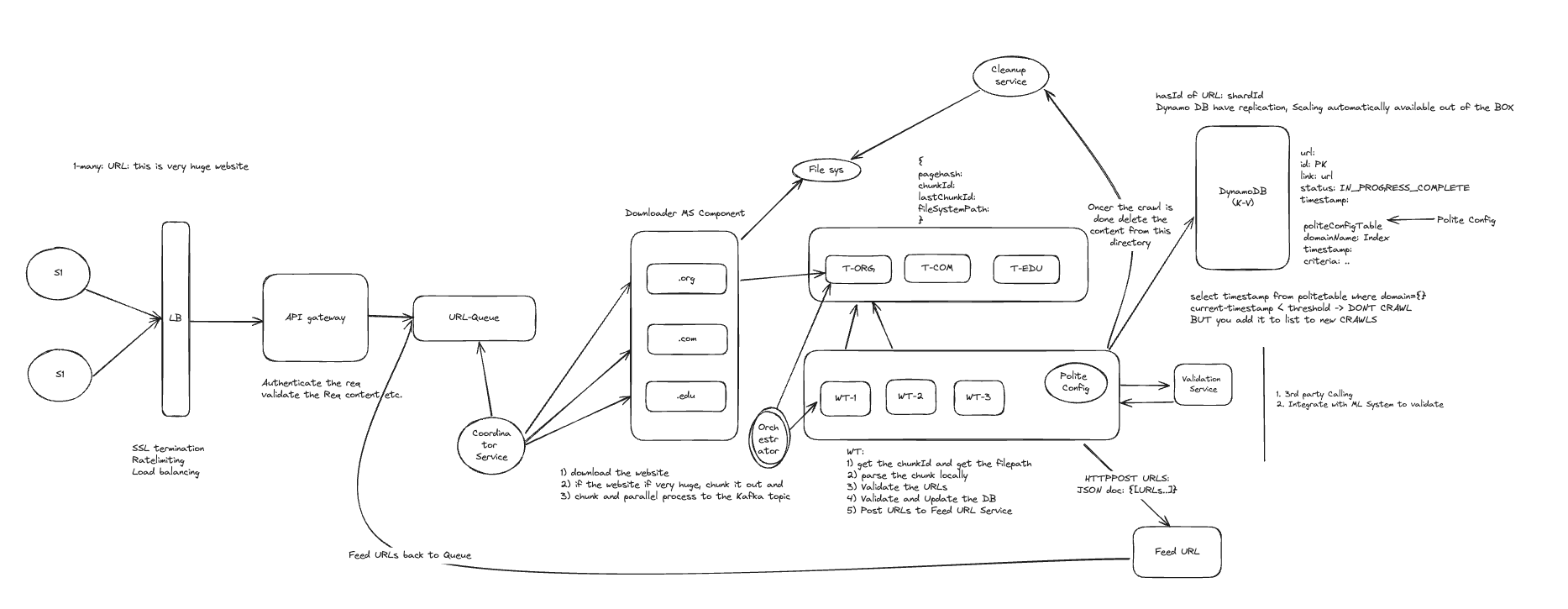
My hand-drawn design for a distributed web crawler.
High-level walkthrough
Admit the seeds. Seed URLs (S1) enter a Load Balancer for SSL termination, rate limiting, and balancing, then pass through an API Gateway that authenticates the request and validates its content.
Queue the graph. Accepted URLs land in a durable URL Queue. One page may fan out to thousands of new URLs, so discovery must be decoupled from downloading.
Coordinate work. A Coordinator Service distributes download jobs across Downloader microservices and sends discovered URLs back toward the queue.
Shard and chunk. Downloaders are sharded by top-level domain — .org, .com, and .edu. Huge sites are chunked for parallel processing; raw bytes go to the File System while metadata records pagehash, chunkId, lastChunkId, and fileSystemPath.
Stream the chunks. Shard-specific Kafka topics — T-ORG, T-COM, and T-EDU — absorb the work. An Orchestrator fans each chunk out to worker tiers WT-1, WT-2, and WT-3.
Process locally. Each worker reads the chunk ID and file path, parses the chunk locally, validates extracted URLs, updates the database, and posts discoveries to the Feed URL service.
Enforce politeness. Polite Config consults the Validation Service for third-party checks and ML URL validation. It reads the domain’s last-crawled timestamp; if now − lastCrawledAt < threshold, do not crawl — park the URL in the new-crawls list for later.
Track crawl state. DynamoDB stores each URL under a URL-hash partition key, distributed by shard ID, with url, id, link, status, and timestamp. Replication and horizontal scaling are managed by the store.
Clean up. After a crawl completes, the Cleanup Service deletes the raw content from its file-system directory.
Close the loop. The Feed URL service posts { "urls": [...] } back into the URL Queue, where dedupe, politeness, and scheduling begin again.
Data model
URL table
PK: hash(url), with shardId for distribution. Attributes: url, id, link, status (IN_PROGRESS or COMPLETE), and timestamp.
PoliteConfig table
Keyed and indexed by domainName. Stores lastCrawledAt, the domain’s crawl-delay threshold, and the next eligible crawl time used to park and release deferred URLs.
Why DynamoDB / NoSQL?
The hot paths are key-value lookups and status writes with no joins. DynamoDB supplies massive write throughput, automatic scaling, built-in replication, and single-digit-millisecond latency. At this volume, a relational design adds write-scaling pressure and schema rigidity without giving the crawler a useful join model.
CAP choice: AP
The crawler favors Availability and Partition tolerance. Work continues through a partition and state converges later. A URL crawled twice is wasted work, not corrupted business data, so eventual consistency is acceptable and URL-hash dedupe remains best effort.
05 / Career
From hands-on engineering to organization-wide leverage.
Staff Engineering Manager · GEICO
Claims engineering · Richardson, Texas
Staff Software Engineer · Meta Platforms
Ads creation and privacy compliance · Mountain View, California
Senior Software Engineer · Twin Health
Mountain View, California
Senior Software Engineer / Team Lead · Werner Enterprises
Omaha, Nebraska
Software Engineer · Robert Bosch
Kalamazoo, Michigan
Software Engineer · Wheaton World Wide
Indianapolis, Indiana
Software Engineer · Gentiva Health Services
Kansas
M.S. Computer Science · Kent State University
B.E. Computer Science · Sri Venkateswara University